NumPy is a Python library that is used for working with arrays. While Python’s lists typically serve the purpose of arrays, they are much slower to process than NumPy’s array object. NumPy’s arrays can be up to 50x faster than traditional Python lists and provide many additional functions that make them particularly useful for data science work.

Why Use NumPy?

NumPy is the key building block of pandas, a Python data analysis library. pandas is a huge part of the Python data viz toolchain and having a basic understanding of NumPy’s core principles can help you get the most out of it.

The benefits of having a good grasp on NumPy fundamentals can also extend into other data science disciplines. In addition to pandas, NumPy’s ecosystem includes SciPy (a library used for scientific computing and technical computing) and scikit-learn (a popular machine learning algorithm library), as well as many other specialized libraries. All of these use NumPy’s multi-dimensional arrays as their primary data objects.

NumPy Setup

Installing NumPy

NumPy should be pre-installed with python distributions such as Anaconda, or can be installed through PIP using the below command:

pip install numpy

Importing NumPy

NumPy is typically imported under the alias np as shown below.

import numpy as np

The NumPy Array

Converting Other Objects into Arrays

Everything in NumPy revolves around its multidimensional array object, ndarray. To create a NumPy ndarray, simply pass a list, tuple, or any array-like object into NumPy’s array() function:

import numpy as np

arr = np.array([1, 2, 3])

Array Properties

The NumPy ndarray has three key properties: its number of dimensions (ndim), shape (shape), and numeric type (dtype). Printing these property values for a standard one-dimensional array will give us the below result:

def print_array_details(a):
	print(f'dimensions: {a.ndim}, shape: {a.shape}, dtype: {a.dtype}')

arr = np.array([1 2 3 4 5 6 7 8])
print_array_details(arr)

# Out: dimensions: 1, shape: (8,), dtype: int64

Dimension refers to the level of array depth or the number of nested arrays. A 0-D array would be an element inside of an array (e.g. 1 from the above arr). The above example is a 1-D array since it is a single array.

We can use the reshape method to change our array into a 2-D array, giving us the below property values:

arr = arr.reshape([2, 4])
print(arr)

# Out: [[1 2 3 4]
# 			[5 6 7 8]]

print_array_details(arr)

# Out: dimensions: 2, shape: (2, 4), dtype: int64

Observing the new values, we can see that we now have 2 dimensions and a shape of (2, 4), letting us know that we have two arrays of four elements each. Our array can be further reshaped into a 3-D array:

arr = arr.reshape([2, 2, 2])
print(arr)

# Out: [[[1 2]
#        [3 4]]
#       [[5 6]
#        [7 8]]]

print_array_details(arr)

# Out: dimensions: 3, shape: (2, 2, 2), dtype: int64

We now have two arrays, each containing two more arrays, with two elements in each array.

Creating Arrays by Shape

NumPy has some utility functions that can be used to create prefilled arrays with a specific shape, without initially specifying array values.

zeros and ones are the most common functions used. The default dtype of these methods is a 64-bit float (float64).

arr = np.zeros([2, 3])
print(arr)

# Out: [[0. 0. 0.] 
#       [0. 0. 0.]]

arr = np.ones([2, 3])
print(arr)

# Out: [[1. 1. 1.] 
#       [1. 1. 1.]]

print(arr.dtype)

# Out: float64

If you want to create an array with random values, you can use the empty method or the random method. The empty method just fills up the necessary memory block with random values, while the random method from NumPy’s random module creates an array with random values between 0 and 1.

arr = np.empty((2, 3))
print(arr)

# Out: [[4.63444165e-310 0.00000000e+000 6.90215607e-310]
#       [6.90216461e-310 6.90216464e-310 6.90216462e-310]]

arr = np.random.random((2, 3))
print(arr)

# Out: [[0.45237836 0.27699219 0.32953788]
#       [0.71824262 0.68951592 0.56671473]]

Finally, linspace and arange can both be used to create arrays with evenly spaced values over a set interval. With linspace, you provide the start number, end number, and number of intervals, whereas arange takes in a start number, end number, and number of steps between each value. linspace array’s datatype is float64 by default.

# 5 numbers in range 2-10
arr = np.linspace(2, 10, 5)
print(arr)

# Out: [ 2.  4.  6.  8. 10.]

# From 2 to 10 (excluding 10) with step size of 2
arr = np.arange(2, 10, 2)

# Out: [2 4 6 8]

Array Indexing and Slicing

One-dimensional arrays are indexed and sliced in a similar manner as Python lists:

arr = np.array([1, 2, 3, 4, 5, 6])

print(arr[2]) 
# Out: 3

print(arr[3:5]) 
# Out: [4 5]

# Every second item from 0-4 set to 0
arr[:4:2] = 0 

print(arr)
# Out: [0 2 0 4 5 6]

# Reverse array
arr = arr[::-1] 

print(arr)
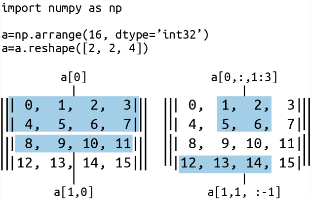
# Out: [6 5 4 0 2 0]

Indexing and slicing multi-dimensional arrays works similarly. Using a comma separated tuple, specify the indexing or slicing operation for each dimension:

arr = np.array([[1, 2, 3, 4], [6, 7, 8, 9]])
print(arr[1, 2])

# Out: 8 (third element of second array)

The below diagram from Data Visualization with Python and JavaScript by Kyran Dale does a great job illustrating the same concept for a 3-D array. Note that, as illustrated in the a[1,0] example, if the number of objects in the selection tuple is less than the number of dimensions, the remaining dimensions are assumed to be fully selected.

Basic Operations

One of the best parts of working with NumPy is that you can perform math operations on arrays as if they were a normal numerical value:

arr = np.array([1, 2, 3, 4])

print(arr + 2)
# Out: [3 4 5 6]

print(arr * 3)
# Out: [3 6 9 12]

Boolean operators work in a similar way. This is used often in pandas to create a Boolean mask.

arr = np.array([3, 5, 19, 6, 12])

print(arr < 10)
# Out: [True True False True False]

NumPy has a ton of basic and advanced mathematical methods that can be applied similarly. Here are some basic examples. A full rundown can be found in NumPy’s documentation.

arr = np.arange(8).reshape((2,4))

print(arr)
# Out: [[0 1 2 3],
#       [4 5 6 7]])

print(arr.min(axis=1))
# Out: [0 4]

print(arr.sum(axis=0))
# Out: [4 6 8 10]

print(arr.mean(axis=1))
# Out: [1.5 5.5]

print(arr.std(axis=1))
# Out: [ 1.11803399 1.11803399]

NumPy also has a bunch of built-in math functions. A few of the more common ones are listed below:

# Trigonometric functions
pi = np.pi
arr = np.array([pi, pi/2, pi/4, pi/6])

# Radians to degrees
print(np.degrees(arr)) 
# Out: [ 180. 90. 45. 30.]

sin_a = np.sin(a)
print(sin_a)
# Out: [1.22464680e-16 1.00000000e+00
#       7.07106781e-01 5.00000000e-01]

# Rounding to 7 decimal places
np.round(sin_a, 7)
# Out: array([ 0.,  1.,  0.7071068,  0.5 ])

# Sums, products, differences
arr = np.arange(8).reshape((2,4))

print(arr)
# Out: [[0 1 2 3]
#       [4 5 6 7]]

# Cumulative sum along second axis
np.cumsum(a, axis=1) 
# Out: [[ 0  1  3  6]
#       [ 4  9 15 22]]

# Without axis argument, array is flattened
np.cumsum(a) 
# Out: [0  1  3  6 10 15 21 28]

Resources

I’d like to give a massive shoutout to the wonderful book, Data Visualization with Python and JavaScript by Kyran Dale. Most of the above examples were from this book and I highly recommend it to anybody looking to improve their data visualization skills using Python and D3.

Some other great resources:

NumPy Documentation

W3 Schools NumPy Tutorial

Real Python NumPy Tutorial

Data Camp NumPy Cheat Sheet